3.2 The Finite Domain Model

The finite domain model is a one-to-one translation of the LP model. Every problem variable of $\mbox{\bf x}$ is represented by a finite domain variable. The inequalities are expressed by appropriate finite domain constraints.

declare 
fun {KnapsackFD Problem}
   NumProducts = {Length Problem.profit}
   Resources   = Problem.resources
in 
   proc {$ Sol}
      sol(maxprofit: MaxProfit = {FD.decl}
          products: Products = {FD.list NumProducts 0#FD.sup})
      = Sol
   in 
      MaxProfit = {FD.sumC Problem.profit Products '=:'}
 
      {ForAll {Arity Resources}
       proc {$ ResourceName}
          Resource = Resources.ResourceName
       in 
          {FD.sumC Resource.npp Products '=<:' Resource.ta}
       end}
 
      {FD.distribute naive Products}
   end 
end

The function KnapsackFD returns a procedure abstracting the script. The solution variable Sol of the script is constrained to a record. The record provides access to the individual quantities of the individual products (under feature products) to obtain a maximum profit (under feature maxprofit).

The variable Products refers to a list of finite domain problem variables (corresponding to $\left[x_1,\ldots,x_n\right]^T$ in the LP model) and MaxProfit is constrained to be the scalar product of the Product variable and the profit vector for the problem specification (see Section 3.1).

The ForAll iterator imposes the inequality constraints $a_{1,i} x_1 + \cdots + a_{n,i} x_n \le b_i$ to the problem variables. The distribution strategy is straightforwardly chosen to naive. Experimenting with first fail (ff) produced even worse results.

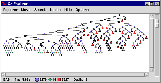
Solving the problem by calling

{ExploreBest {KnapsackFD Problem} proc {$ O N} O.maxprofit <: N.maxprofit end}

produces the following search tree.