10.2 Example: Locating Warehouses

This example features branch and bound to compute an optimal solution, a non-trivial distribution strategy and symbolic constraints.

Problem Specification

Assume a company which wants to construct warehouses to supply stores with goods. Each warehouse to be constructed would have a certain capacity defining the largest number of stores which can be supplied by this warehouse. For the construction of a warehouse we have fixed costs. The costs for transportation from a warehouse to a store vary depending on the location of the warehouse and the supplied store. The aim is to determine which warehouses should be constructed and which stores should be supplied by the constructed warehouses such that the overall costs are minimized.

We assume the fixed costs of building a warehouse to be 50. We furthermore assume 5 warehouses W1 through W5 and 10 stores Store1 through Store10. The capacities of the warehouses are shown in Figure 10.2. The costs to supply a store by a warehouse are shown in Figure 10.3.


Capacity	1	4	2	1	3

Figure 10.2: Capacities of warehouses.


${\it Store}_1$	36	42	22	44	52
${\it Store}_2$	49	47	134	135	121
${\it Store}_3$	121	158	117	156	115
${\it Store}_4$	8	91	120	113	101
${\it Store}_5$	77	156	98	135	11
${\it Store}_6$	71	39	50	110	98
${\it Store}_7$	6	12	120	98	93
${\it Store}_8$	20	120	25	72	156
${\it Store}_9$	151	60	104	139	77
${\it Store}_{10}$	79	107	91	117	154

Figure 10.3: Costs for supplying stores.

Model

We assume that the costs are given in the matrix CostMatrix defined by Figure 10.3. For the model of this problem we introduce the following variables.

${\it Open}_i, 1 \leq i \leq 5$ , with domain $0\#1$ such that ${\it Open}_i=1$ if warehouse does supply at least one store.
${\it Supplier}_i, 1 \leq i \leq 10$ , with domain $1\#5$ such that ${\it Supplier}_i = j$ if store ${\it Store_i}$ is supplied by warehouse .
${\it Cost}_i, 1 \leq i \leq 10$ , such that the domain of ${\it Cost}_i$ is defined by the row ${\it CostMatrix}_i$ . The variable ${\it Cost}_i$ denotes the costs of supplying store ${\it Store}_i$ by warehouse $W_{{\it Supplier}_i}$ , i. e., ${\it Cost}_i = {\it CostMatrix}_{i,{\it Supplier}_i}$ .

We have the additional constraint that the capacity of the warehouses must not be exceeded. To this aim we introduce auxiliary variables ${\it Supplies}_{i,j}$ with the domain $0\#1$ as follows.

$\forall i \in \{1,\ldots,5\} \forall j \in \{1,\ldots, 10\}:\ ({\it Supplies}_{i,j} = 1) \leftrightarrow ({\it Supplier_j} = i)$

The capacity constraints can then be stated with

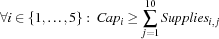
$\forall i \in \{1, \ldots, 5\}:\ {\it Cap}_i \geq \sum\limits_{j=1}^{10}{\it Supplies}_{i,j}$

where ${\it Cap}_i$ is defined according to Figure 10.2.

Distribution Strategy

There are several possibilities to define a distribution strategy for this problem.

least regret

We choose to determine the variables ${\it Cost}_i$ by distribution. Because no entry in a row of the cost matrix occurs twice, we immediately know which store is supplied by which warehouse. We select the variable ${\it Cost}_i$ first for which the difference between the smallest possible value and the next higher value is maximal. Thus, decisions are made early in the search tree where the difference between two costs by different suppliers are maximal. The distribution strategy will try the minimal value in the domain of ${\it Cost}_i$ first. In Operations Research this strategy is known as the principle of least regret.

Script

The script in Figure 10.4 constrains its root variable to a record containing the supplying warehouse for each store, the costs for each store to be supplied by the corresponding warehouse and the total costs.

The statement

{FD.element Supplier.St CostMatrix.St Cost.St}

connects the costs to supply a store with the supplier. Because no element in a row of the cost matrix occurs twice, the supplier for a store is known if its costs are determined and vice versa. Through this statement the constraint ${\it Cost}_i = {\it CostMatrix}_{i,{\it Supplier}_i}$ is imposed.

A propagator for the constraint that the capacity of a warehouse is not exceeded can be created by the statement

{FD.atMost Capacity.S Supplier S}

The statement

Open.S = {FD.reified.sum {Map Stores fun {$ St} Supplier.St =: S end} '>:' 0}

guarantees that a variable ${\it Open}_i$ in the model is constrained to 1 if warehouse W_i supplies at least one store.

The first solution of the problem can be found with the statement

{ExploreOne WareHouse}

To compute the solution with minimal costs we define the following ordering relation.

proc {Order Old New}  
   Old.totalCost >: New.totalCost  
end

The optimal solution with total cost 604 can now be computed with

{ExploreBest WareHouse Order}

Capacity   = supplier(3 1 4 1 4)
CostMatrix = store(supplier(36 42 22 44 52)  
                   supplier(49 47 134 135 121)  
                   supplier(121 158 117 156 115)  
                   supplier(8 91 120 113 101)  
                   supplier(77 156 98 135 11)  
                   supplier(71 39 50 110 98)  
                   supplier(6 12 120 98 93)  
                   supplier(20 120 25 72 156)  
                   supplier(151 60 104 139 77)  
                   supplier(79 107 91 117 154))
BuildingCost = 50
fun {Regret X}
   M = {FD.reflect.min X}  
in  
   {FD.reflect.nextLarger X M} - M
end 
proc {WareHouse X}
   NbSuppliers = {Width Capacity}
   NbStores    = {Width CostMatrix}
   Stores      = {List.number 1 NbStores 1}
   Supplier    = {FD.tuple store NbStores 1#NbSuppliers}
   Open        = {FD.tuple supplier NbSuppliers 0#1}
   Cost        = {FD.tuple store NbStores 0#FD.sup}
   SumCost     = {FD.decl} = {FD.sum Cost '=:'}
   NbOpen      = {FD.decl} = {FD.sum Open '=:'}
   TotalCost   = {FD.decl}
in 
   X = plan(supplier:Supplier cost:Cost totalCost:TotalCost)
   TotalCost =: SumCost + NbOpen*BuildingCost
   {For 1 NbStores 1
    proc {$ St}
       Cost.St :: {Record.toList CostMatrix.St}
       {FD.element Supplier.St CostMatrix.St Cost.St}
    end}
   {For 1 NbSuppliers 1
    proc {$ S}  
       {FD.atMost Capacity.S Supplier S}
       Open.S = {FD.reified.sum {Map Stores fun {$ St}  
                                               Supplier.St =: S  
                                            end} '>:' 0}
    end}
   {FD.distribute
    generic(order: fun {$ X Y} {Regret X} > {Regret Y} end)
    Cost}
end

Figure 10.4: A script for the warehouse problem.